Problem 3 - Answers
In the problem, we will be once again building on the simulation developed in the previous problems. We will be taking advantage of our approach of simulating particles at discrete time steps to add in other kinds of forces on particles.
a) One type of force commonly considered in simulating macroparticles is drag. Modify your step function to add an additional ‘Stokes drag’ force on each particle:
Animate your simulation to see how adding drag impacts your simulation.
%matplotlib inline
import numpy as np
import matplotlib.pyplot as plt
from matplotlib.animation import FuncAnimation
from scipy.spatial.distance import pdist,squareform
from IPython.display import HTML
import time
dt = 0.001
A = 1
B = 10
K = 0.1
L = 0.1
g = 10.0
def initialise(n,stdev=1.0):
poslist = []
vellist = []
n_upper = np.ceil(np.sqrt(n))
for i in range(n):
poslist.append(1/(n_upper+1)*np.array([i//n_upper+1,i%n_upper+1]))
vellist.append(np.random.normal(0.0,stdev,size=(2)))
pos = np.array(poslist)
vel = np.array(vellist)
return pos,vel
def step(n,pos,vel):
dX = np.zeros((n,n))
dY = np.zeros((n,n))
for i in range(1,n):
dX.flat[i:n*(n-i):n+1] = (pos[:n-i,0] - pos[i:,0]).flat
dY.flat[i:n*(n-i):n+1] = (pos[:n-i,1] - pos[i:,1]).flat
# calculate distances and get the matrix of force magnitudes
norms = np.sqrt(dX**2 + dY**2)
C = np.zeros((n,n))
C[norms!=0] = -1 / norms[norms!=0]**3 * np.exp(-norms[norms!=0]/K)
# multiply displacements by force magnitudes to get force vectors
dX *= C
dY *= C
# make the matrices antisymmetric
dX += -1 * np.rot90(np.fliplr(dX))
dY += -1 * np.rot90(np.fliplr(dY))
# Sum particle-particle forces to get 2D force vector
Fip = np.vstack([np.sum(dX,axis=0),np.sum(dY,axis=0)]).T
# Calculate forces due to walls at X=0,1 and Y=0,1
FW = B*(np.exp((-pos)/L)/(pos)**2 - np.exp((pos-1)/L)/(pos-1)**2)
# Calculate the drag force
FD = -g * vel
# Euler step
vel += (Fip + FW + FD) * dt
pos += vel * dt
return pos,vel
def animate(pos,vel,n,nstep,interval=20):
fig,ax = plt.subplots()
plt.close(fig)
ax.set_aspect(aspect=1.0)
ln, = ax.plot(pos[:,0],pos[:,1],'ro')
data = []
for i in range(nstep):
pos,vel = step(n,pos,vel)
data.append(pos.copy())
def init():
ax.set_xlim(0,1)
ax.set_ylim(0,1)
return ln,
def update(i):
ln.set_data(data[i][:,0],data[i][:,1])
return ln,
anim = FuncAnimation(fig,update,frames=range(nstep),init_func=init,blit=True,interval=interval)
return HTML(anim.to_jshtml())
pos,vel = initialise(100)
animate(pos,vel,n=100,nstep=1000,interval=100)
b) You’ll have noticed that a drag force causes the particles to slowly lose energy until they come to rest. This is not physical - the fluctuation-dissipation theorem says that the physical process causing drag, or ‘dissipation’ (in this case, collision with microparticles) will also cause a ‘fluctuation’. In the case of a macroparticle in a fluid, this is Brownian motion.
Add Brownian motion to your simulation. This can be represented as a force term which, at each time step, is randomly sampled from a 2D Gaussian distribution. Look up the Langevin equation for more details on this.
Make an animation and observe the effects.
T = 100.0
def step(n,pos,vel):
dX = np.zeros((n,n))
dY = np.zeros((n,n))
for i in range(1,n):
dX.flat[i:n*(n-i):n+1] = (pos[:n-i,0] - pos[i:,0]).flat
dY.flat[i:n*(n-i):n+1] = (pos[:n-i,1] - pos[i:,1]).flat
# calculate distances and get the matrix of force magnitudes
norms = np.sqrt(dX**2 + dY**2)
C = np.zeros((n,n))
C[norms!=0] = -1 / norms[norms!=0]**3 * np.exp(-norms[norms!=0]/K)
# multiply displacements by force magnitudes to get force vectors
dX *= C
dY *= C
# make the matrices antisymmetric
dX += -1 * np.rot90(np.fliplr(dX))
dY += -1 * np.rot90(np.fliplr(dY))
# Sum particle-particle forces to get 2D force vector
Fip = np.vstack([np.sum(dX,axis=0),np.sum(dY,axis=0)]).T
# Calculate forces due to walls at X=0,1 and Y=0,1
FW = B*(np.exp((-pos)/L)/(pos)**2 - np.exp((pos-1)/L)/(pos-1)**2)
# Calculate the drag force
FD = -g * vel
# Apply Brownian 'kick'
FB = np.random.normal(0.0,T,size=(n,2))
# Euler step
vel += (Fip + FW + FD + FB) * dt
pos += vel * dt
return pos,vel
pos,vel = initialise(100)
animate(pos,vel,n=100,nstep=1000,interval=100)
c) Changing the standard deviation of the Gaussian Brownian noise, you are effectively modifying the ‘temperature’ of the particle system. Repeat your animation with different ‘temperatures’ and note the effect.
T = 10.0
pos,vel = initialise(100)
animate(pos,vel,n=100,nstep=1000,interval=100)
T = 30.0
pos,vel = initialise(100)
animate(pos,vel,n=100,nstep=1000,interval=100)
T = 300.0
pos,vel = initialise(100)
animate(pos,vel,n=100,nstep=1000,interval=100)
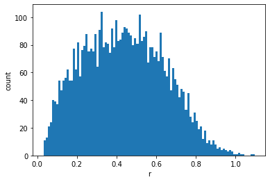
d) Clearly, the particle system is more ‘disordered’ at higher temperatures. A good way of visualising the order of a particle system is to plot its correlation function. Make and compare plots of the correlation function for different temperatures.
pos,vel = initialise(100)
T = 10.0
for i in range(1000):
pos,vel = step(100,pos,vel)
plt.hist(pdist(pos),bins=100)
plt.xlabel('r')
plt.ylabel('count')
Text(0, 0.5, 'count')
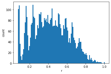
pos,vel = initialise(100)
T = 30.0
for i in range(1000):
pos,vel = step(100,pos,vel)
plt.hist(pdist(pos),bins=100)
plt.xlabel('r')
plt.ylabel('count')
Text(0, 0.5, 'count')
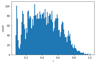
pos,vel = initialise(100)
T = 100.0
for i in range(1000):
pos,vel = step(100,pos,vel)
plt.hist(pdist(pos),bins=100)
plt.xlabel('r')
plt.ylabel('count')
Text(0, 0.5, 'count')
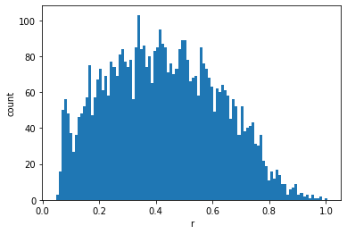
pos,vel = initialise(100)
T = 300.0
for i in range(1000):
pos,vel = step(100,pos,vel)
plt.hist(pdist(pos),bins=100)
plt.xlabel('r')
plt.ylabel('count')
Text(0, 0.5, 'count')