Problem 3¶

In this first part we’ll learn to solve differential equations numerically in Python. In the second part we’ll use the code we write here to solve a much more complicated problem. As a motivating example, we will be proving Kepler’s first law numerically.

The force on a body of mass $m$ at $\boldsymbol{\mathrm{r}}$ due to a body of mass $M$ at the origin is given by Newton’s law

$\boldsymbol{\mathrm{F}}= -\frac{GMm}{\left|\boldsymbol{r}\right|^3}\boldsymbol{r}$

In two dimensions, where $\boldsymbol{\mathrm{r}}=x\boldsymbol{\hat{\imath}} + y \boldsymbol{\hat{\jmath}}$ , the components of the acceleration $\boldsymbol{\mathrm{a}}=a_x \boldsymbol{\hat{\imath}} + a_y \boldsymbol{\hat{\jmath}}$ are given by

$a_x = \frac{\mathrm{d}v_x}{\mathrm{d}t} = - \frac{GMx}{\left(x^2 + y^2\right)^{3/2}},\quad a_y = \frac{\mathrm{d}v_y}{\mathrm{d}t} = - \frac{GMy}{\left(x^2 + y^2\right)^{3/2}}$

A problem where we know the equations of motion and the starting point for the system is called an initial value problem and is a very common numerical problem in physics. Python comes with a few ways to easily solve initial value problems. Here we’ll use the scipy.integrate.solve_isp function.

We have to provide the function with three arguments to work (see the documentation for more). The first argument is a function $\boldsymbol{\mathrm{F}}(t,\boldsymbol{\mathrm{X}})$ which ‘updates’ the system, this is where the equations of motion are set. This function must take the time, and a state vector as inputs and return the derivative (wrt time) of the state vector’s components. Our state vector we’ll call $\boldsymbol{\mathrm{X}}$ and which just holds the current state of the system, in our case

$\boldsymbol{\mathrm{X}} = \left(x, y, v_x, v_y\right)$

So it follows that the function $\boldsymbol{\mathrm{F}}(t,\boldsymbol{\mathrm{X}})$ must return

$\boldsymbol{\mathrm{F}}(t,\boldsymbol{\mathrm{X}}) = \left(v_x, v_y, a_x, a_y\right)$

The first two components are simply the last two components in the input. The second two components can be calculated from the acceleration equations above. The other arguments that scipy.integrate.solve_isp requires is the initial state of the system $\boldsymbol{\mathrm{X}}_0$ and the time span over which to solve the equations.

A few tips:

You must set the method argument of solve_isp to ”Radau” to get a stable solution.
Set the t_eval to an array of time coordinates and the function will find $\boldsymbol{\mathrm{X}}$ at those time coordinates.
The $(x, y, v_x, v_y)$ values are stored in array at result.y where result = solve_isp(…)

Example: Kepler’s First Law¶

States that

All planets move in elliptical orbits, with the sun at one focus.

To prove this numerically, start the solver with a body at $x=1 \mathrm{AU}$ , $y=0$ and an initial velocity $35$ km/s in the positive $y$ direction. Plot the $x$ and $y$ values and you should see an elliptical orbit. Ensure you run the simulation over a sensible time-scale, e.g. a few years.

Now check if the orbit is elliptical. The equation of an ellipse is $ $\frac{x^2}{a^2} + \frac{y^2}{b^2} = 1$ $where$ a $and$ b $are the semi-minor and semi-major axes respectively. What are$ a $and$ b$ for this orbit? The below figure shows what the orbit should look like.

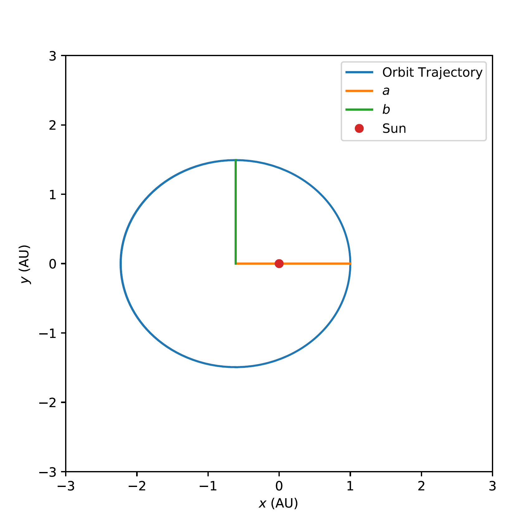
Fig. 1 The elliptical orbit for the Kepler’s law example.¶

Hint

Rearrange the above to something that looks like the equation for a straight line and fit to find $a$ and $b$ . The $x$ and $y$ in the equation are centred on the centre of the ellipse but our data is centred on the sun (the ellipse’s focus). Make sure to shift your data (only necessary in $x$ ) to the centre.

PyProblems

Problem 3¶

Example: Kepler’s First Law¶